How to Calculate Pay Back Period in Excel

You'd be surprised how simple the calculations are that sophisticated investors rely on. Payback period is one such example.

Payback period is a calculation of how much time it takes to make your money back from an investment. Investors have their tolerance for how long they're willing to wait for a return, and this is all they need to make a decision.

The odd thing is there isn't built in functionality for this in Excel, so I'm going to show you how to make a nifty little spreadsheet that automatically updates when you change the variables.

In order to make this work, we're going to combine use of the following formulas

• Index
• If
• Countif
• Abs
• Sum

The most important thing here is the setup of the data that you already have i.e. the initial investment/cash outlay and the future cash flows by period.

To do this, you put your initial investment in one row and your future cash flows in another row.

Next, you sum up the total cash flow for each period.

After that, you add a row to capture the cumulative cash flow. This formula should equal cumulative cash flow from the prior period plus the cash flow from the current period.

If you do this correctly, you should have a cumulative cash flow row, with some negative rows and some positive rows. In most projects, you expected to see some ramp up of positive cash flows once you make an initial investment. Your file should look something like this one (I'll tell you about the last row in a minute.):

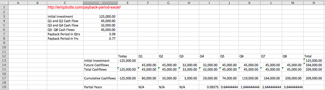
Now, to the tricky parts…automating determining the payback period. You can break the payback period equation down into two parts: a) full years with negative cumulative cash flow and b) the partial year where the project breaks even.

So to count the number of years with negative cash flow, you use the COUNTIF formula. In this case, the formula was COUNTIF(F17:M17,"<0″).

For the partial year, you have to take a couple of steps. Now is when we talk about the last row from the screen shot above. First, you need to create that by using the IF and ABS formulas together. In my example, I typed =IF(F17<0,"N/A",ABS(E17)/F15) into the first payback period and then copied and pasted in all of the payback periods to the right. Abs formula takes the absolute value of the selected argument so that we can determine what % of the year it took to offset the cumulative negative value.

The next thing you need to do is use the COUNTIF and the INDEX formulas together. By using the formula INDEX(F19:M19,,COUNTIF(F17:M17,"<0″)+1). That formula equates to "give me the first number in the last row where the cumulative cash flow is not zero.

So by adding INDEX(F19:M19,,COUNTIF(F17:M17,"<0″)+1) and COUNTIF(F17:M17,"<0″), you get a formula for payback period that will change dynamically based on the values you input.

Bonus tip: whenever possible link your tables to a single input so that updating the data is much simpler. In this case. I linked the relevant values to the data table at the top of the screen.

Click the button below if you want to see the video of how to do this. I'll also send you the Excel file for you to play around with. If you've already joined my free content library, you can get the video and Excel file here.

How to Calculate Pay Back Period in Excel

Source: https://getgoodatexcelfast.com/blog/payback-period-excel

Share this post